Fine-tuning a VLM on TextVQA

This example walks through a vision-language model (VLM) fine-tuning pipeline for TextVQA, where the task is to answer questions that require reasoning over text inside an image. The base model is Qwen2.5-VL-3B-Instruct, fine-tuned with the QLoRA method. The data backbone is one Lance table that evolves from raw multimodal rows into training-ready features. The key idea is simple: in this QLoRA fine-tuning setup, we freeze the VLM’s image encoder and train only a small adapter on the language-model side. We call that encoder the vision tower in this example: it is the part of the model that turns image pixels into visual hidden states before the language model reads them alongside the text prompt. Because the vision tower’s weights do not change during fine-tuning, its output for a given image also does not change. That means the pipeline can compute those visual hidden states once, store them as a fixed-size Lance column, and reuse them in every epoch instead of recomputing them in every training step. This also helps the run fit comfortably on a small GPU, because the training job does not need to keep the vision encoder active or pay for its forward pass on every batch.

Open the Colab demo

Run the Colab-sized workflow on a free T4: download the pre-baked Lance subset, explore it, benchmark Lance vs Parquet, fine-tune with QLoRA, and evaluate base vs tuned answers.

View the full demo source

Full demo repository with the notebook, Geneva UDFs, direct backfill fallback, dataloader, training loop, and evaluation scripts.

The Colab notebook uses a pre-baked subset of the TextVQA dataset: it downloads a curated Lance subset whose expensive feature columns have already been computed. This page explains the complete end-to-end pipeline that produced that subset, then shows how the notebook applies it to produce a fine-tuned model that improves performance on the TextVQA task.

What you get

On the curated text_dense TextVQA slice, the demo fine-tunes Qwen2.5-VL-3B-Instruct with QLoRA and evaluates on held-out images:

Setup	TextVQA accuracy
Base model	0.799
LoRA-tuned model	0.820
Lift	+2.1 percentage points

The larger point is not the absolute score, because you could just as well fine-tune a better base model on more data. The main takeaways are the workflow and quality-of-life improvements that you get when you combine LanceDB and Geneva:

Add expensive features as new columns without rewriting the raw dataset.
Read fixed-size model features efficiently for shuffled PyTorch batches.
Iterate quickly from feature idea to scalable CPU/GPU backfill, using Geneva UDFs.

Why LanceDB fits this workflow

VLM fine-tuning pipelines spend a lot of time between “I have an experiment idea” and “I trained the model.” LanceDB shortens that loop in three places.

Cheap feature evolution

Lance can append derived columns such as ocr_token_count, dhash, vision_tower_hiddens, and tokenized SFT prompts without rewriting the existing image/question/answer columns or managing sidecar files.

Efficient training reads

Lance is optimized for scans and random access over fixed-size lists, which are common in model training: embeddings, hidden states, token IDs, masks, and labels.

Fast experiment turnaround

Geneva lets AI engineers express feature work as UDFs, run those UDFs across CPU or GPU workers, and materialize the results directly into the same Lance table.

In this pipeline, those three properties combine into the core optimization: compute the VLM vision features once, store them cheaply, then train by reading only the cached columns the model needs.

Pipeline overview

The runnable demo uses the exact Colab subset hosted at lance-format/textvqa-lance-colab. It is derived from the Lance-formatted TextVQA corpus and stores inline JPEG bytes, questions, answers, OCR tokens, object classes, CLIP image/question embeddings, and the cached training features used by this example. The full demo pipeline adds three tiers of derived features on top.

Tier 1: text features

Cheap CPU columns such as question_length, answer_length, question_type, and ocr_token_count.

Tier 2: light image features

Image-derived columns such as dhash, computed by decoding the JPEG once and storing a perceptual hash.

Tier 3: VLM training features

GPU-heavy columns: vision_tower_hiddens plus SFT token fields (input_ids, attention_mask, labels).

The Colab notebook’s workflow starts after all three tiers have been computed. It downloads a small curated subset and runs the training/evaluation path without needing to run Geneva or the vision-tower backfill on the notebook GPU.

1. Start with a multimodal LanceDB table

The base schema comes from the TextVQA Lance dataset. One row contains the image bytes, natural-language question, reference answers, OCR tokens, scene tags, and retrieval embeddings.

Python

import pyarrow as pa

BASE_SCHEMA = pa.schema([
    pa.field("id",            pa.int64()),
    pa.field("image",         pa.large_binary()),
    pa.field("image_id",      pa.string()),
    pa.field("question_id",   pa.string()),
    pa.field("question",      pa.string()),
    pa.field("answers",       pa.list_(pa.string())),
    pa.field("answer",        pa.string()),
    pa.field("image_emb",     pa.list_(pa.float32(), 512)),
    pa.field("question_emb",  pa.list_(pa.float32(), 512)),
    pa.field("ocr_tokens",    pa.list_(pa.string())),
    pa.field("image_classes", pa.list_(pa.string())),
    pa.field("set_name",      pa.string()),
])

Because the raw image, text, OCR, and embedding features live together, the same table supports curation, retrieval, feature engineering, and training. For example, the notebook can run a text-to-image retrieval demo by searching image_emb with a question embedding that already exists in the row.

2. Add feature columns with Geneva

Geneva turns feature engineering into UDF definitions plus backfills. The UDFs can be simple text functions, image-processing functions, or stateful GPU model calls. The Tier 1 features are ordinary CPU UDFs:

Python

import re
import pyarrow as pa
from geneva.transformer import udf

_QUESTION_TYPE_PATTERNS = [
    ("how_many", re.compile(r"^\s*how\s+many\b", re.IGNORECASE)),
    ("what_brand", re.compile(r"^\s*what\s+(is\s+the\s+)?(brand|company|make)\b", re.IGNORECASE)),
    ("what", re.compile(r"^\s*what\b", re.IGNORECASE)),
]

@udf(data_type=pa.string(), input_columns=["question"])
def question_type(question: str) -> str:
    for label, pattern in _QUESTION_TYPE_PATTERNS:
        if pattern.search(question or ""):
            return label
    return "other"

@udf(data_type=pa.int32(), input_columns=["ocr_tokens"])
def ocr_token_count(ocr_tokens: list[str] | None) -> int:
    return len(ocr_tokens) if ocr_tokens else 0

The Tier 3 feature is heavier: run Qwen2.5-VL’s frozen vision tower once, then store the merged visual hidden states as a fixed-size fp16 list.

Python

IMAGE_PX = 560
LLM_TOKENS_PER_IMAGE = 400
VISION_HIDDEN = 2048

@udf(
    data_type=pa.list_(pa.float16(), LLM_TOKENS_PER_IMAGE * VISION_HIDDEN),
    input_columns=["image"],
)
class VisionTowerEmbedder:
    def __init__(self):
        self._model = None
        self._processor = None

    def _lazy_load(self):
        if self._model is not None:
            return
        import torch
        from transformers import AutoProcessor, Qwen2_5_VLForConditionalGeneration

        self._torch = torch
        self._model = Qwen2_5_VLForConditionalGeneration.from_pretrained(
            "Qwen/Qwen2.5-VL-3B-Instruct",
            torch_dtype=torch.bfloat16,
            device_map="cuda:0",
        ).model.visual.eval()
        self._processor = AutoProcessor.from_pretrained("Qwen/Qwen2.5-VL-3B-Instruct")

    def __call__(self, image: bytes) -> list[float]:
        self._lazy_load()
        # Decode image, resize to IMAGE_PX, run the frozen vision tower,
        # and return fp16[400, 2048] flattened as one fixed-size list.
        ...

The fixed shape matters. With IMAGE_PX = 560, Qwen2.5-VL produces 400 merged visual tokens, each with hidden size 2048. That becomes one fp16[400 * 2048] column per row. Training can scan and randomly access that column without decoding images or running the vision tower in the hot loop, saving GPU compute at training time. Run the tiered backfill with Geneva:

bash

python -m vlm.backfill_geneva --tier 1     # CPU text columns
python -m vlm.backfill_geneva --tier 2     # image decode + dhash
python -m vlm.backfill_geneva --tier 3     # vision tower + SFT tokens

The same Tier 3 work can be done manually by creating PyArrow batches and calling Lance’s column-evolution APIs directly. The demo repo includes backfill_direct.py for that path. Geneva is the preferred abstraction when you want to scale the same feature code across CPU or GPU workers and keep backfills incremental.

See the full UDF registry in vlm/geneva_udfs.py and the backfill driver in vlm/backfill_geneva.py.

3. Curate a training slice

The demo uses a text_dense slice: TextVQA examples whose images contain many OCR tokens. The slice was chosen empirically because it gave the clearest LoRA lift over the already-strong base model.

Python

TEXT_DENSE_OCR_THRESHOLD = 16

def matches_text_dense(row: dict) -> bool:
    return len(row.get("ocr_tokens") or []) >= TEXT_DENSE_OCR_THRESHOLD

The Colab-ready bake ingests a small train split, backfills Tier 3 on that train table, ingests a held-out validation split, and optionally pushes the result to Hugging Face:

bash

python -m vlm.colab_prepare \
  --out data/colab \
  --slice text_dense \
  --train-rows 600 \
  --val-rows 400 \
  --hf-repo lance-format/textvqa-lance-colab \
  --push

The train table contains cached Tier 3 columns because training reads them directly. The validation table keeps raw images because evaluation should run the full VLM on unseen images.

4. Explore the prepared table

Before training, it helps to look at the actual task. Each row pairs an image with a question whose answer is often visible as text in the image: a product label, phone screen, sign, book spine, or package.

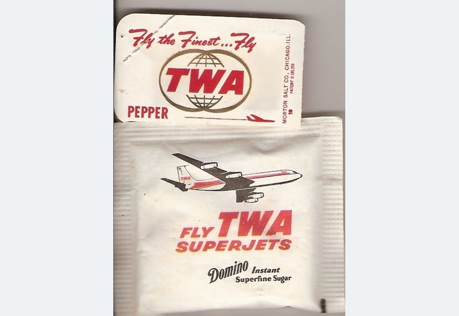
Q: what is the name of the airline on the sugar packet?

A: TWAOCR: 7h the Finest… 74 1E TWA 8 SALT REESE PEPPER

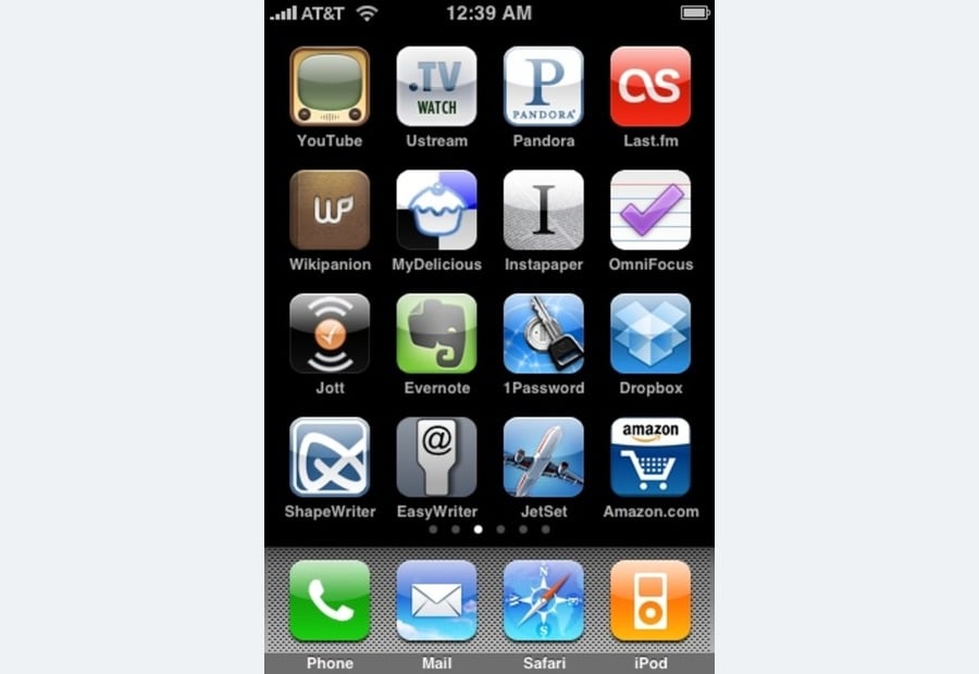
Q: what time is displayed?

A: 12:39 amOCR: AT&T 12:39 AM TV CS WATCH P PANDORA YouTube Ustream

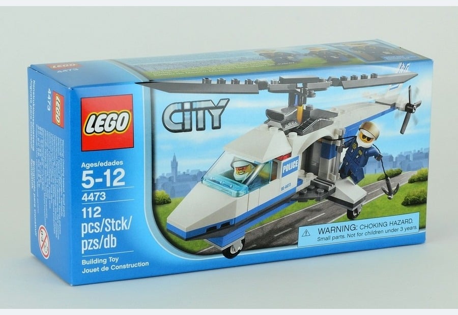
Q: what brand of building block is this?

A: legoOCR: LEGO CITY Ages/edades 5-12 POLICE B-403 4473 112 112 pcs

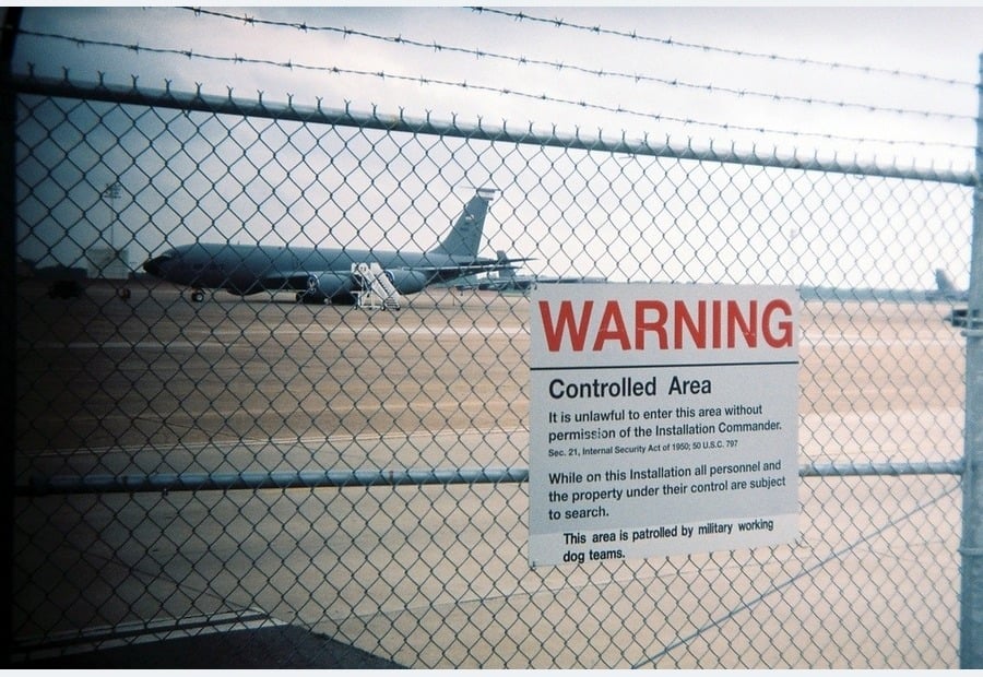
Q: what is printed in red?

A: warningOCR: WARNING Controlled Area Itis unlawf enter thisre without permission nstallation

The notebook downloads the public pre-baked subset:

Python

from huggingface_hub import snapshot_download
import lancedb
import os

local = snapshot_download(
    repo_id="lance-format/textvqa-lance-colab",
    repo_type="dataset",
    local_dir="data/colab",
)

def open_tbl(path: str):
    name = os.path.basename(path).removesuffix(".lance")
    return lancedb.connect(os.path.dirname(path)).open_table(name)

train_tbl = open_tbl(f"{local}/textvqa_colab_train.lance")
val_tbl = open_tbl(f"{local}/textvqa_colab_val.lance")

Because the table also ships CLIP embeddings, you can run cross-modal retrieval without loading a model:

Python

import numpy as np

seed = (
    train_tbl.search()
    .select(["question", "question_emb"])
    .limit(40)
    .to_arrow()
    .to_pylist()[11]
)

hits = (
    train_tbl.search(
        np.asarray(seed["question_emb"], dtype=np.float32),
        vector_column_name="image_emb",
    )
    .select(["image", "question", "answer", "_distance"])
    .limit(5)
    .to_arrow()
    .to_pylist()
)

This is the same table that later feeds training. There is no separate feature store, image directory, Parquet export, or manifest to keep synchronized.

5. Benchmark Lance vs Parquet-style reads

Many training pipelines start with Parquet. Parquet is excellent for columnar analytics, but training commonly needs shuffled batches and fixed-size tensor columns. The notebook compares Lance and Parquet on two access patterns:

Column group	Why it matters
`image`, `question`, `answer`	Raw multimodal rows: the baseline “decode and tokenize during training” path.
`vision_tower_hiddens`	Cached fixed-size fp16 VLM features: the optimized training path.

The notebook mirrors those column groups to uncompressed Parquet, then measures sequential scans and shuffled random batches:

Python

RAW = ["image", "question", "answer"]
VEC = ["vision_tower_hiddens"]
BATCH = 8

lance_ds = train_tbl.to_lance()
n = train_tbl.count_rows()

def seq(ds, cols):
    t0 = time.time()
    for _ in ds.to_batches(columns=cols, batch_size=BATCH):
        pass
    return n / (time.time() - t0)

def shuf(ds, cols, num_batches=20):
    batches = [
        sorted(rng.choice(n, BATCH, replace=False).tolist())
        for _ in range(num_batches)
    ]
    t0 = time.time()
    for idx in batches:
        ds.take(idx, columns=cols)
    return (num_batches * BATCH) / (time.time() - t0)

One Colab run produced the following throughput:

Throughput, rows/s	LanceDB	Parquet
`image` + `question` + `answer`, sequential	2,603	8,311
`image` + `question` + `answer`, shuffled	2,613	352
`vision_tower_hiddens` fp16, sequential	1,452	90
`vision_tower_hiddens` fp16, shuffled	2,149	—

The takeaways are workload-specific:

For a traditional sequential scan over raw image/question/answer columns, Parquet is faster in this run: 8,311 rows/s vs 2,603 rows/s.
For shuffled raw multimodal batches, Lance is faster because training reads scattered rows repeatedly instead of streaming the file once.
For cached fp16 fixed-size arrays, Lance is about 16x faster than Parquet on the sequential scan. This is the training-relevant path in this example: the model reads vision_tower_hiddens, token IDs, masks, and labels as fixed-size columns.
The benchmark intentionally skips the Parquet fp16 shuffled case. Parquet would re-decode whole row groups for each random batch, which is slow enough to distract from the real use case. The sequential fp16 row already shows the layout gap, while Lance shuffled reads remain fast.

The numbers shown above are central to the example. The Tier 3 feature is only useful if the storage format can read it efficiently in the way a trainer actually needs: projected columns, repeated scans, and shuffled batches. Lance specializes in exactly that access pattern, including fixed-size list columns stored on disk.

6. Load cached columns with the Permutation API

The training DataLoader projects only the columns needed by the cached training loop:

Python

from lancedb.permutation import Permutation

CACHED_COLS = [
    "vision_tower_hiddens",
    "input_ids",
    "attention_mask",
    "labels",
]

class LancePermutationDataset(torch.utils.data.Dataset):
    def __init__(self, uri: str, table_name: str):
        self.uri = uri
        self.table_name = table_name
        self._perm = None
        self.length = len(lancedb.connect(uri).open_table(table_name))

    def __len__(self):
        return self.length

    def __getstate__(self):
        state = self.__dict__.copy()
        state["_perm"] = None
        return state

    def _ensure_open(self):
        if self._perm is None:
            tbl = lancedb.connect(self.uri).open_table(self.table_name)
            self._perm = (
                Permutation.identity(tbl)
                .select_columns(CACHED_COLS)
                .with_format("arrow")
            )

    def __getitems__(self, indices: list[int]):
        self._ensure_open()
        return self._perm.__getitems__(indices)

Each worker opens its own Permutation, reads Arrow batches directly from Lance, and avoids per-row Python object conversion until the collate function converts arrays into tensors. The training batch contains:

Field	Shape
`vision_hiddens`	`fp16[B, 400, 2048]`
`input_ids`	`int64[B, 512]`
`attention_mask`	`int64[B, 512]`
`labels`	`int64[B, 512]`

7. Fine-tune without loading the vision tower

The training process loads the language-model side of Qwen2.5-VL in 4-bit, deletes the vision tower, and wraps the LLM projections with LoRA adapters. During the forward pass, the model embeds the token IDs, finds the <|image_pad|> positions, and inserts the cached visual hidden states into those positions:

Python

def forward_cached(model, batch, image_pad_id: int):
    base = model.get_base_model() if hasattr(model, "get_base_model") else model
    inner = base.model

    inputs_embeds = inner.get_input_embeddings()(batch.input_ids)
    _, _, hidden_dim = inputs_embeds.shape

    mask = (
        (batch.input_ids == image_pad_id)
        .unsqueeze(-1)
        .expand_as(inputs_embeds)
    )

    vision_flat = batch.vision_hiddens.to(inputs_embeds.dtype).reshape(-1, hidden_dim)
    inputs_embeds = inputs_embeds.masked_scatter(mask, vision_flat)

    return model(
        inputs_embeds=inputs_embeds,
        attention_mask=batch.attention_mask,
        labels=batch.labels,
    ).loss

At this point, the LanceDB integration is done. The rest is plain PyTorch: optimizer, gradient accumulation, checkpointing, and saving the LoRA adapter.

Python

loader = make_cached_loader(
    "data/colab/textvqa_colab_train.lance",
    batch_size=2,
    shuffle=True,
)

for batch in loader:
    batch = batch.to(device)
    loss = forward_cached(model, batch, image_pad_id)
    (loss / grad_accum).backward()
    ...

This produces a training log like the following. The loss falls as the adapter learns from the cached features, and peak VRAM stays at 5.3 GB because QLoRA trains without keeping the vision tower active:

step  10/300  loss=2.6694  5.9 samples/s
step  20/300  loss=2.3133  6.1 samples/s
                 .
                 .
                 .
step 290/300  loss=0.0359  6.3 samples/s
step 300/300  loss=0.4750  6.3 samples/s
saved adapter to runs/colab_lora/lora | peak VRAM 5.3 GB

The training loop pays zero per-step cost for image decode, vision-tower forward, or prompt tokenization. Those costs were moved into feature engineering, where LanceDB and Geneva make them durable, incremental, and reusable.

8. Evaluate on held-out images

Evaluation uses the held-out validation table and loads the full VLM, including the vision tower. That is intentional: inference should see raw unseen images, not the cached train features.

Python

rows = (
    val_tbl.search()
    .select(["image", "question", "answer", "answers"])
    .limit(256)
    .to_arrow()
    .to_pylist()
)

base_model, processor = load_model(adapter_dir=None, load_4bit=True)
tuned_model, processor = load_model(adapter_dir="runs/colab_lora/lora", load_4bit=True)

base_score = score_textvqa(base_model, processor, rows)
tuned_score = score_textvqa(tuned_model, processor, rows)

In this end-to-end example, the held-out curated validation split produced:

Model	TextVQA accuracy
Base `Qwen2.5-VL-3B-Instruct`	0.799
QLoRA-tuned adapter	0.820
Lift	+2.1 percentage points

The tuned adapter is not meant to be a state-of-the-art TextVQA checkpoint. It is the proof point for the pipeline: the same Lance table supports curation, feature engineering, efficient training reads, and evaluation on held-out raw images. The notebook renders side-by-side examples: image, question, base answer, tuned answer, and ground truth. This closes the loop from feature idea to trained model while keeping the source data, derived features, training batches, and evaluation split in Lance.

Full source

The complete demo implementation with helper scripts and usage instructions is in this repo.

Notebook

The runnable Colab workflow: download, explore, benchmark, train, and evaluate.

Geneva UDFs

Tier 1, Tier 2, and Tier 3 feature definitions.

Backfill driver

Geneva-powered feature materialization.

Training loop

QLoRA training from cached Lance columns.

Open the Colab demo

View the full demo source

​What you get

​Why LanceDB fits this workflow

Cheap feature evolution

Efficient training reads

Fast experiment turnaround

​Pipeline overview

Tier 1: text features

Tier 2: light image features

Tier 3: VLM training features

​1. Start with a multimodal LanceDB table

​2. Add feature columns with Geneva

​3. Curate a training slice

​4. Explore the prepared table

Q: what is the name of the airline on the sugar packet?

Q: what time is displayed?

Q: what brand of building block is this?

Q: what is printed in red?

​5. Benchmark Lance vs Parquet-style reads

​6. Load cached columns with the Permutation API

​7. Fine-tune without loading the vision tower

​8. Evaluate on held-out images

​Full source

Notebook

Geneva UDFs

Backfill driver

Training loop

What you get

Why LanceDB fits this workflow

Pipeline overview

1. Start with a multimodal LanceDB table

2. Add feature columns with Geneva

3. Curate a training slice

4. Explore the prepared table

5. Benchmark Lance vs Parquet-style reads

6. Load cached columns with the Permutation API

7. Fine-tune without loading the vision tower

8. Evaluate on held-out images

Full source