This example walks through fine-tuning an autonomous vehicle (AV) perception model on targeted failure-mode slices of BDD100K — riders, nighttime pedestrians, and distant pedestrians — using LanceDB as a single multimodal table from raw JPEG bytes through to the PyTorch training loop.
The full pipeline lives in the lancedb/training repository. This page focuses on the parts most relevant to training: defining curated splits as materialized views, loading them through the Permutation API, and pinning checkpoints to an exact data version.
What you get
Fine-tuning Faster R-CNN ResNet50 FPN v2 for 10 epochs on each curated slice (batch size 64, AMP, A100), starting from the same COCO-pretrained checkpoint and evaluating on the matching validation view:
| Failure mode | Metric | Baseline (COCO) | Fine-tuned | Δ% |
|---|
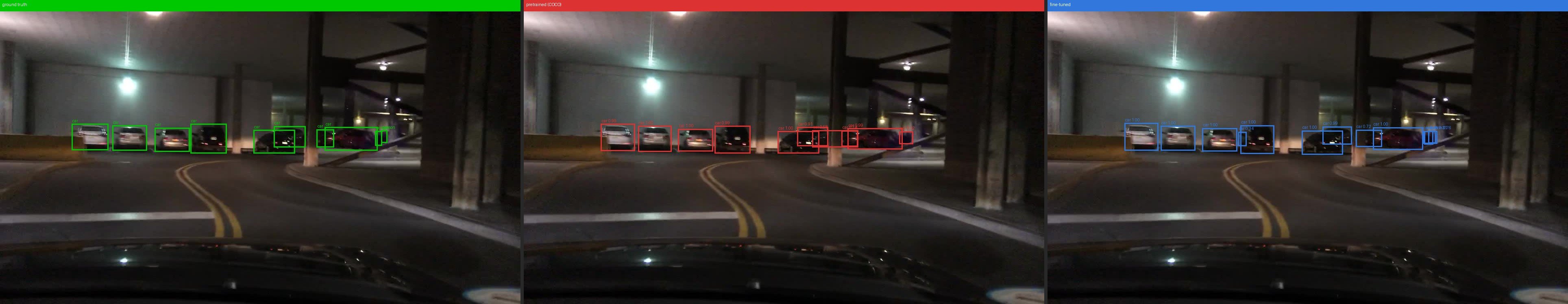
| Nighttime pedestrian | mAP@0.5 | 0.4025 | 0.5192 | +29.0% |
| Recall | 0.5923 | 0.7570 | +27.8% |
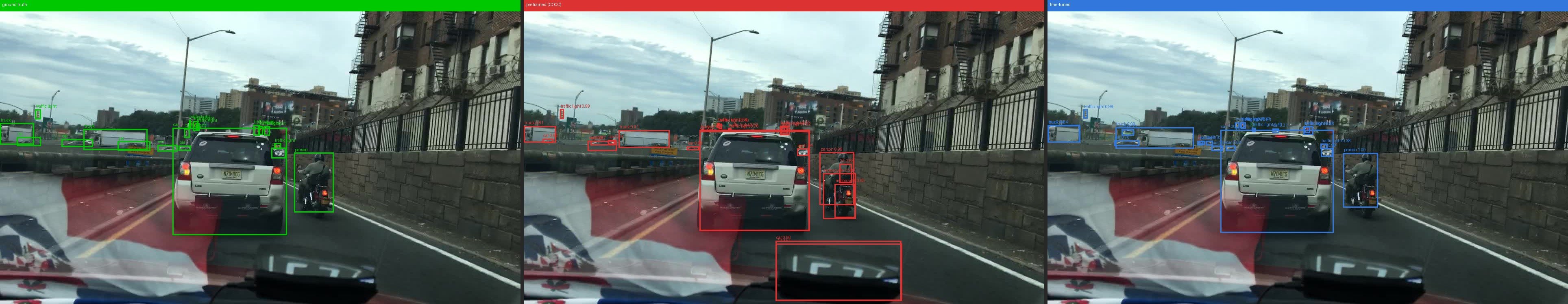
| Rider | mAP@0.5 | 0.5563 | 0.6676 | +20.0% |
| Recall | 0.6788 | 0.7847 | +15.6% |
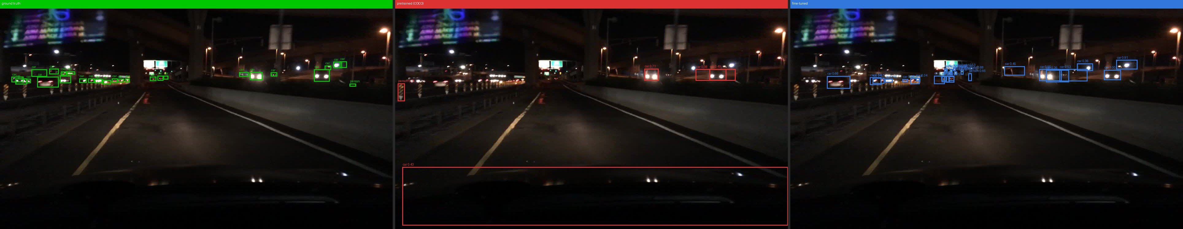
| Distant pedestrian | mAP@0.5 | 0.4746 | 0.5788 | +22.0% |
| Recall | 0.6794 | 0.8024 | +18.1% |
 The rest of the page walks through the pipeline that produced these checkpoints.
The failure modes
A perception model fine-tuned on a generic dataset typically misses the long-tail scenarios that matter most in deployment. Three common failure modes drive this example:
| Failure mode | Curation signal |
|---|
| Riders (person on bike/motorcycle) | has_rider = true |
| Nighttime pedestrians | timeofday = 'night' AND has_person = true |
| Distant pedestrians | has_person = true AND person_bbox_area_pct < 30.0 |
add() → backfill() → refresh(); no manifests, no exports, no reshuffling on disk.
1. Schema
The source table holds raw image bytes alongside structured annotations. Bounding boxes are stored as a parallel list (one element per box) rather than a nested struct so they remain directly queryable with SQL.
import pyarrow as pa

BDD_SCHEMA = pa.schema([
    pa.field("image_id",   pa.string()),
    pa.field("split",      pa.string()),         # "train" | "val"
    pa.field("image_bytes", pa.large_binary()),  # raw JPEG
    pa.field("width",      pa.int32()),
    pa.field("height",     pa.int32()),

    # scene metadata
    pa.field("weather",    pa.string()),
    pa.field("scene",      pa.string()),
    pa.field("timeofday",  pa.string()),

    # annotations — parallel lists, one element per box
    pa.field("ann_categories", pa.list_(pa.string())),
    pa.field("ann_bboxes",     pa.list_(pa.list_(pa.float32()))),
    pa.field("ann_occluded",   pa.list_(pa.bool_())),
])
pa.RecordBatches of raw frames + annotations directly into a Lance table — no intermediate preprocessing job. The table can live on local disk, S3, GCS, or Azure; everything downstream (backfills, views, the training loader) opens it in place via lancedb.connect("s3://...") with no local copy step.
2. Backfill curation features with Geneva
Curation signals are added as columns on the same table using Geneva UDFs. Backfills are incremental and checkpointed: re-running the command after new footage arrives only computes the new rows.
import pyarrow as pa
from geneva.transformer import udf

# Tier 1 — CPU, derived from annotations alone
@udf(data_type=pa.bool_(), input_columns=["ann_categories"])
def has_rider(ann_categories: list[str]) -> bool:
    return "rider" in (ann_categories or [])

# Tier 2 — GPU, runs a Faster R-CNN to find the largest detected person
# as a percentage of frame area. <30% = a distant or small pedestrian,
# the hard case we want to upweight in training.
@udf(data_type=pa.float32(),
     input_columns=["image_bytes", "width", "height"],
     cuda=True, num_gpus=1)
class PersonBboxAreaPct:
    def __init__(self):
        self._model = None

    def __call__(self, image_bytes, width, height):
        # lazy model load — runs once per Ray worker, then reused
        ...
import geneva

gconn = geneva.connect("data/bdd100k/lancedb")
tbl   = gconn.open_table("bdd100k")

tbl.add_columns({"has_rider": has_rider})
tbl.add_columns({"person_bbox_area_pct": PersonBboxAreaPct()})

with gconn.local_ray_context():
    tbl.backfill("has_rider")
    tbl.backfill("person_bbox_area_pct")
Because the curation features are flat scalar columns on the same table, all four retrieval modes — SQL, full-text search, vector search, and SQL-filtered vector search — work directly without joins or exports. See the Geneva end-to-end example for more on the backfill pattern. 3. Define training splits as materialized views
A training split is a named SQL filter, not a CSV manifest. Each view stays in sync with the source table and bumps its version on every refresh — the link between a checkpoint and the exact data that produced it.
import geneva

gconn = geneva.connect("data/bdd100k/lancedb")
gtbl  = gconn.open_table("bdd100k")

VIEWS = {
    "bdd100k_rider_train":
        "has_rider = true AND split = 'train'",
    "bdd100k_rider_val":
        "has_rider = true AND split = 'val'",
    "bdd100k_nighttime_person_train":
        "timeofday = 'night' AND has_person = true AND split = 'train'",
    "bdd100k_nighttime_person_val":
        "timeofday = 'night' AND has_person = true AND split = 'val'",
    "bdd100k_distant_person_train":
        "has_person = true AND person_bbox_area_pct < 30.0 AND split = 'train'",
    "bdd100k_distant_person_val":
        "has_person = true AND person_bbox_area_pct < 30.0 AND split = 'val'",
}

with gconn.local_ray_context():
    for name, sql_filter in VIEWS.items():
        query = gtbl.search().where(sql_filter)
        mv = gconn.create_materialized_view(name, query)
        mv.refresh()
        print(f"[{name}]  {mv.count_rows()} rows  (version {mv.version})")
4. PyTorch DataLoader via the Permutation API
The training script doesn’t know about the filter — it opens a view by name and reads through the Permutation API. Each DataLoader worker reopens its own connection lazily, reads Arrow batches directly from Lance (zero-copy, no intermediate file format), and the collate function decodes the whole batch in one pass. Permutation provides random-access indexing over the table, so shuffling is a cheap pointer rewrite rather than a full-dataset shuffle on disk.
import lancedb
import torch
import torchvision.io as tio
from lancedb.permutation import Permutation

DETECTION_COLS = ["image_bytes", "ann_categories", "ann_bboxes"]

class LanceDetectionDataset(torch.utils.data.Dataset):
    def __init__(self, uri: str, table_name: str):
        self.uri, self.table_name = uri, table_name
        self._perm = None
        self.length = len(lancedb.connect(uri).open_table(table_name))

    def __len__(self):
        return self.length

    def __getstate__(self):
        # Permutation holds Rust async state — zero it so each worker reopens
        state = self.__dict__.copy()
        state["_perm"] = None
        return state

    def _ensure_open(self):
        if self._perm is None:
            tbl = lancedb.connect(self.uri).open_table(self.table_name)
            self._perm = (
                Permutation.identity(tbl)
                .select_columns(DETECTION_COLS)
                .with_format("arrow")  # zero-copy
            )

    def __getitems__(self, indices: list[int]):
        self._ensure_open()
        return self._perm.__getitems__(indices)
BDD_LABEL_MAP = {
    "person": 1, "rider": 1, "bicycle": 2, "car": 3, "motorcycle": 4,
    "bus": 6, "train": 7, "truck": 8, "traffic light": 10,
}


def detection_collate(batch):
    images, targets = [], []
    for raw, cats, bboxes in zip(
        batch.column("image_bytes").to_pylist(),
        batch.column("ann_categories").to_pylist(),
        batch.column("ann_bboxes").to_pylist(),
    ):
        buf = torch.frombuffer(bytearray(raw), dtype=torch.uint8)
        images.append(tio.decode_image(buf, tio.ImageReadMode.RGB).float() / 255.0)

        valid_boxes, valid_labels = [], []
        for cat, box in zip(cats or [], bboxes or []):
            lid = BDD_LABEL_MAP.get(cat)
            if lid is None or box[2] <= box[0] or box[3] <= box[1]:
                continue
            valid_boxes.append(box)
            valid_labels.append(lid)
        targets.append({
            "boxes":  torch.tensor(valid_boxes  or [], dtype=torch.float32).reshape(-1, 4),
            "labels": torch.tensor(valid_labels or [], dtype=torch.int64),
        })
    return images, targets
torch.utils.data.DataLoader:
def make_loader(uri, table_name, batch_size=64, num_workers=8, shuffle=False):
    dataset = LanceDetectionDataset(uri, table_name)
    sampler = torch.utils.data.RandomSampler(dataset) if shuffle else None
    return torch.utils.data.DataLoader(
        dataset,
        batch_size=batch_size,
        sampler=sampler,
        num_workers=num_workers,
        collate_fn=detection_collate,
        pin_memory=torch.cuda.is_available(),
        persistent_workers=(num_workers > 0),
        multiprocessing_context="spawn" if num_workers > 0 else None,
    )
with_format("arrow") keeps batches as zero-copy pa.RecordBatches — no per-row Python boxing, no pickling between worker and main. Each DataLoader worker reopens its own Permutation after fork (the Rust async handle is cleared in __getstate__), so reads scale with num_workers and stream straight from the underlying object store. JPEG decode overlaps with GPU compute via pin_memory + prefetch_factor, which is what keeps the loader from becoming the bottleneck on a fast GPU.
5. Fine-tune Faster R-CNN
The training loop is plain PyTorch — the Lance integration ends at the loader. Mixed precision is enabled on CUDA for ~2× speedup on Ampere GPUs.
import time
import torch
from torchvision.models.detection import (
    fasterrcnn_resnet50_fpn_v2, FasterRCNN_ResNet50_FPN_V2_Weights,
)

device  = torch.device("cuda" if torch.cuda.is_available() else "cpu")
use_amp = device.type == "cuda"

# COCO pretrained weights — head left intact since BDD uses a subset of COCO IDs
model = fasterrcnn_resnet50_fpn_v2(
    weights=FasterRCNN_ResNet50_FPN_V2_Weights.COCO_V1
).to(device)

train_loader = make_loader("data/bdd100k/lancedb",
                           "bdd100k_rider_train",
                           batch_size=64, num_workers=14, shuffle=True)
val_loader   = make_loader("data/bdd100k/lancedb",
                           "bdd100k_rider_val",
                           batch_size=64, num_workers=14)

optimizer = torch.optim.SGD(
    [p for p in model.parameters() if p.requires_grad],
    lr=0.04, momentum=0.9, weight_decay=1e-4,
)
scheduler = torch.optim.lr_scheduler.StepLR(optimizer, step_size=3, gamma=0.1)
scaler    = torch.cuda.amp.GradScaler() if use_amp else None

for epoch in range(1, 11):
    model.train()
    t0 = time.time()
    for images, targets in train_loader:
        images  = [img.to(device) for img in images]
        targets = [{k: v.to(device) for k, v in t.items()} for t in targets]
        if all(t["labels"].numel() == 0 for t in targets):
            continue

        with torch.cuda.amp.autocast(enabled=use_amp):
            losses = sum(model(images, targets).values())

        optimizer.zero_grad()
        if use_amp:
            scaler.scale(losses).backward()
            scaler.unscale_(optimizer)
            torch.nn.utils.clip_grad_norm_(model.parameters(), 10.0)
            scaler.step(optimizer)
            scaler.update()
        else:
            losses.backward()
            torch.nn.utils.clip_grad_norm_(model.parameters(), 10.0)
            optimizer.step()

    scheduler.step()
    print(f"epoch {epoch}  ({time.time() - t0:.1f}s)")
6. Pin the checkpoint to a data version
Every Lance table — including a materialized view — exposes a monotonically increasing version. Logging it next to the weights gives a permanent, deterministic link between a checkpoint and the exact data snapshot that produced it.
import json
from pathlib import Path

train_tbl = lancedb.connect("data/bdd100k/lancedb").open_table("bdd100k_rider_train")

out = Path("checkpoints/rider")
out.mkdir(parents=True, exist_ok=True)
torch.save(model.state_dict(), out / "fasterrcnn_bdd_finetuned.pt")
with open(out / "metadata.json", "w") as f:
    json.dump({
        "train_table":   train_tbl.name,
        "table_version": train_tbl.version,
        "row_count":     len(train_tbl),
    }, f, indent=2)
tbl = lancedb.connect("data/bdd100k/lancedb").open_table("bdd100k_rider_train")
tbl.checkout(version=7)   # exact snapshot the checkpoint was trained on
7. Continuous updates
When new footage arrives, the same three calls update every downstream view — no view definitions change, no training-script edits required:
# 1. ingest the new footage into the source table
table.add(new_record_batches)

# 2. backfill computes only the new rows (incremental, checkpointed)
with gconn.local_ray_context():
    tbl.backfill("has_rider")
    tbl.backfill("person_bbox_area_pct")

# 3. refresh appends qualifying new rows to every materialized view
for view_name in gconn.table_names():
    if view_name == "bdd100k":
        continue
    mv = gconn.open_table(view_name)
    before = mv.count_rows()
    mv.refresh()
    print(f"[{view_name}]  {before} → {mv.count_rows()} rows  (version {mv.version})")
version.
Full source
The complete code, including a synthetic-data mode for pipeline verification (--synthetic 500), GPU UDFs for CLIP embeddings and dHash deduplication, and the EDA notebook, is in this GitHub repository.