Finding the Needle in a Haystack: Comparing Multi-vector Search Strategies

In the development of advanced search and retrieval systems, moving from keyword matching to semantic understanding is a critical step. However, a key distinction exists between finding a relevant document and locating a specific piece of information within that document with precision. While there are techniques that perform well for retrieving documents, most of them work by extracting summarized semantic meaning of the document. This can be seen as these models trying to understand the “gist” of the documents. Both single-vector search and late-interaction approaches work well for these conditions with various tradeoffs involved. But there’s another type of problem where the goal is not just to understand the overall topic of a document in general, but to also specifically account for the requested detail within the document. This “needle in a haystack” problem is a significant challenge, and addressing it is essential for building high-precision retrieval systems. This guide provides a technical analysis of multivector search for high-precision information retrieval. We will examine various optimization strategies and analyze their performance. This guide should be seen as complementary to resources like this blog post by Answer.AI on ColBERT pooling, which explains how pooling strategies can be effective for document-level retrieval. Here, we will demonstrate why those same techniques can be counterproductive when precision at an intra-document, token level is the primary objective. To reproduce the work below, see the code here.

The Dataset

This task is different from benchmarks like BEIR, which focus on text-based doc retrieval, finding the most relevant documents from a large collection. Here, we want intra-document localization, where the goal is to find a precise piece of information within a single, dense document, in a multimodal setting.

The Task: The Document Haystack Dataset

Our benchmark is built on the AmazonScience/document-haystack dataset, which contains 25 visually complex source documents (e.g., financial reports, academic papers). To create a rigorous test, our evaluation follows a per-document methodology:

We process each of the 25 source documents independently.
Table Creation: For a single source document (e.g., “AIG”), we ingest all pages from all of its page-length variants (from 5 to 200 pages long). This creates a temporary LanceDB table containing approximately 1,230 pages.
The Task: We then query this table using a set of “needle” questions, where the goal is to retrieve the exact page number containing the answer. A successful retrieval means the correct page number is within the top K results.
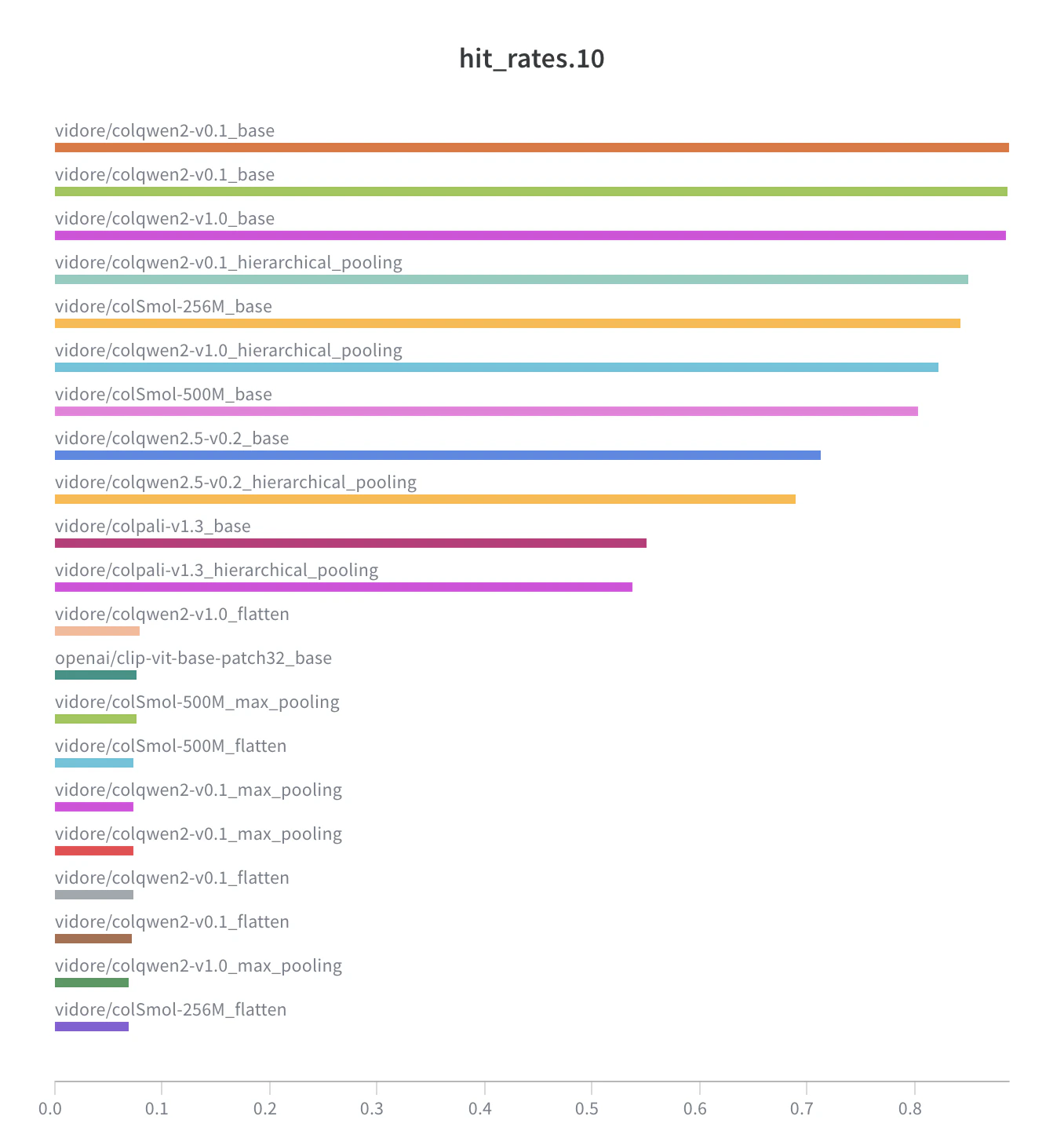
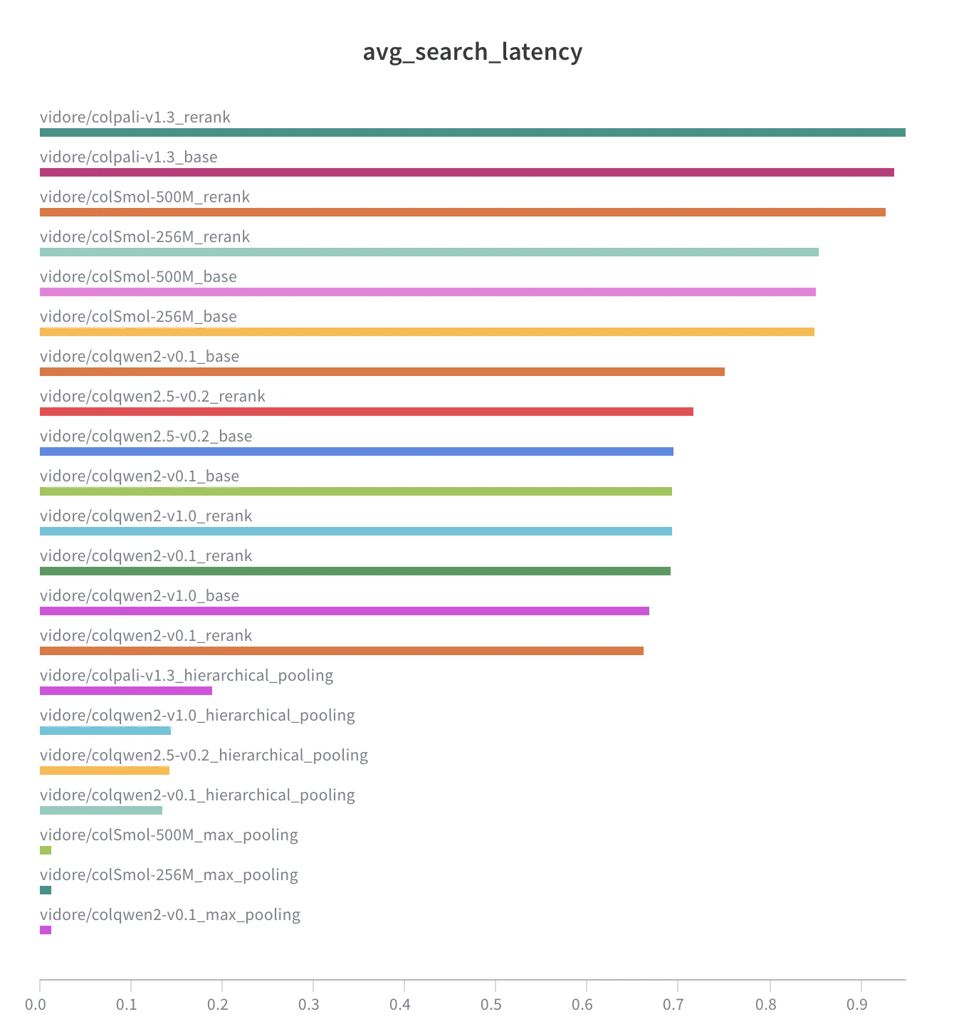
Target metric: We measure both retrieval accuracy (Hit@K) and the average search latency for each query against this table.

Dataset example The documents contain “text needles” like these

During evaluation, the queries processed are somewhat like this:

What is the secret currency in the document?
What is the secret object #3 in the document?

The intention of this task is to find the page which has the text needle that answers this questions

Models and Architectures

Our testbed includes a baseline single-vector model and a family of advanced multivector models.

Single-Vector (Bi-Encoder) Baseline: `openai/clip-vit-base-patch32`

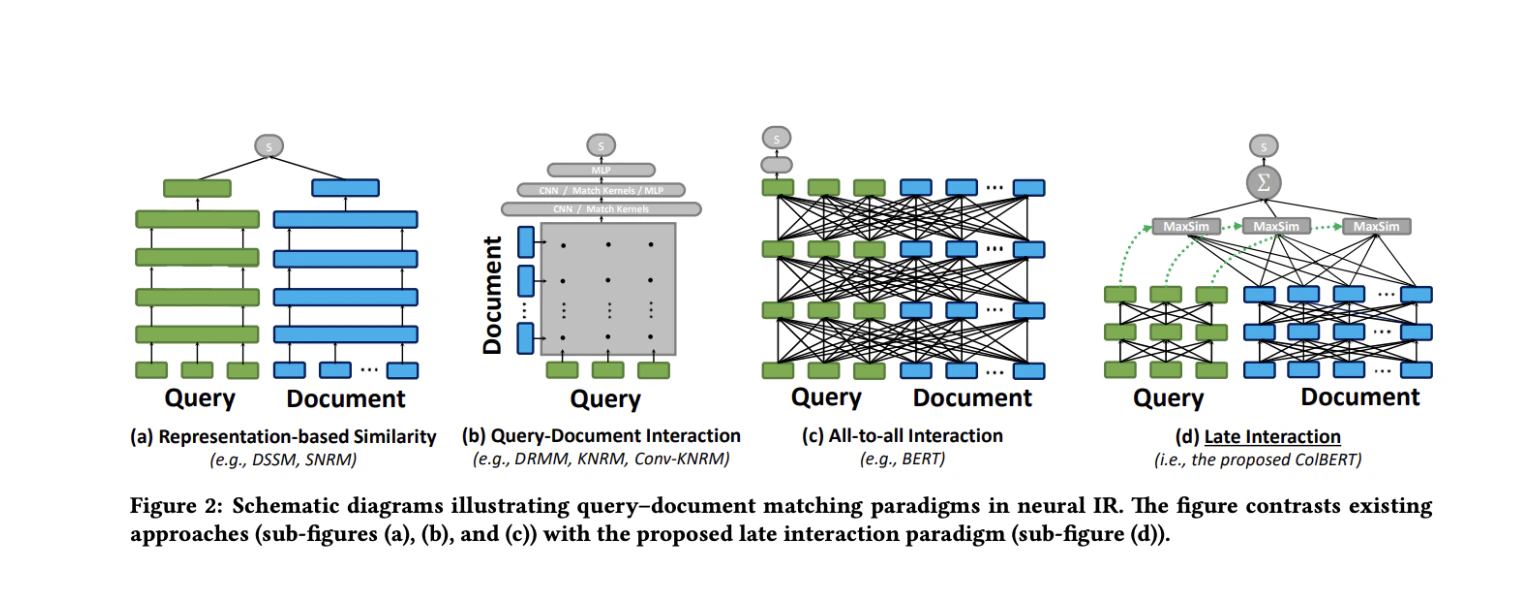
A bi-encoder maps an entire piece of content (a query, a document page) to a single vector. The search process is simple: pre-compute one vector for every page, and at query time, find the page vector closest to the query vector.

Strength: Speed and simplicity.
Weakness: This creates an information bottleneck. All the nuanced details, keywords, and semantic relationships on a page must be compressed into a single, fixed-size vector. For finding a needle, this is like trying to describe a specific person’s face using only one word.

Multi-vector (Late-Interaction) Models

Multi-vector models, pioneered by ColBERT, take a different approach. Instead of one vector per page, they generate a set of vectors for each page—one for every token (or image patch).

Mechanism (MaxSim): The search process is more sophisticated. For each token in the query, the system finds the most similar token on the page. These maximum similarity scores are then summed up to get the final relevance score. This “late-interaction” preserves fine-grained, token-level details.
The Models: We used several vision-language models adapted for this architecture, including ColPali, ColQwen2, and ColSmol. While their underlying transformer backbones differ, they all share the ColBERT philosophy of representing documents as a bag of contextualized token embeddings.

Different Retrieval Strategies Used

A full multivector search is powerful but computationally intensive. Here are five strategies for managing it, complete with LanceDB implementation details.

1. `base`: The Gold Standard (Full Multi-vector Search)

This is the pure, baseline late-interaction search. It offers the highest potential for accuracy by considering every token. LanceDB also integrates with ConteXtualized Token Retriever (XTR) , an advanced retrieval model that prioritizes the most semantically important document tokens during search. This integration enhances the quality of search results by focusing on the most relevant token matches. LanceDB Implementation:

Python

import lancedb
import pyarrow as pa

# Schema for multivector data
# Assumes embeddings are 128-dimensional
schema = pa.schema([
    pa.field("page_num", pa.int32()),
    pa.field("vector", pa.list_(pa.list_(pa.float32(), 128)))
])

db = lancedb.connect("./lancedb")
tbl = db.create_table("document_pages_base", schema=schema)

# Ingesting multi-token embeddings for a page
# multi_token_embeddings is a NumPy array of shape (num_tokens, 128)
tbl.add([{"page_num": 1, "vector": multi_token_embeddings.tolist()}])

# Searching with a multi-token query
# query_multi_vector is also shape (num_query_tokens, 128)
results = tbl.search(query_multi_vector).limit(5).to_list()

2. `flatten`: Mean Pooling

This strategy “flattens” the set of token vectors into a single vector by averaging them. This transforms the search into a standard, fast approximate nearest neighbor (ANN) search. LanceDB Implementation:

Python

# Schema for single-vector data
schema_flat = pa.schema([
    pa.field("page_num", pa.int32()),
    pa.field("vector", pa.list_(pa.float32(), 128))
])
tbl_flat = db.create_table("document_pages_flat", schema=schema_flat)

# Ingesting the mean-pooled vector
mean_vector = multi_token_embeddings.mean(axis=0)
tbl_flat.add([{"page_num": 1, "vector": mean_vector.tolist()}])

# Searching with a single averaged query vector
query_mean_vector = query_multi_vector.mean(axis=0)
results = tbl_flat.search(query_mean_vector).limit(5).to_list()

3. `max_pooling`

This is a variation of flatten. max_pooling takes the element-wise max across all token vectors instead of the mean. The implementation is identical to flatten, just with a different aggregation method (.max(axis=0)).

4. `flatten and multivector rerank`: The Hybrid “Optimization”

This two-stage strategy aims for the best of both worlds. First, use a fast, pooled-vector search to find a set of promising candidates. Then, run the full, accurate multivector search on only those candidates. LanceDB Implementation: This requires a table with two vector columns.

Python

# Schema with both flat and multivector columns
schema_rerank = pa.schema([
    pa.field("page_num", pa.int32()),
    pa.field("vector_flat", pa.list_(pa.float32(), 128)),
    pa.field("vector_multi", pa.list_(pa.list_(pa.float32(), 128)))
])
tbl_rerank = db.create_table("document_pages_rerank", schema=schema_rerank)

# Ingest both vectors
tbl_rerank.add([
    {
        "page_num": 1,
        "vector_flat": multi_token_embeddings.mean(axis=0).tolist(),
        "vector_multi": multi_token_embeddings.tolist()
    }
])

# --- Two-Stage Search ---
# Stage 1: Fast search on the flat vector
query_flat = query_multi_vector.mean(axis=0)
candidates = tbl_rerank.search(query_flat, vector_column_name="vector_flat") \
                       .limit(100) \
                       .with_row_id(True) \
                       .to_pandas()

# Stage 2: Precise multivector search on candidates
candidate_ids = tuple(candidates["_rowid"].to_list())
final_results = tbl_rerank.search(query_multi_vector, vector_column_name="vector_multi") \
                          .where(f"_rowid IN {candidate_ids}") \
                          .limit(5) \
                          .to_list()

5. `hierarchical token pooling`: Compressing the Haystack

This is an indexing-time strategy that aims to reduce the storage footprint and computational cost of multivector search by reducing the number of vectors per document. Instead of using every token vector, it clusters semantically similar tokens together and replaces them with a single, averaged vector.

Mechanism: For each document, it computes the similarity between all token vectors, performs hierarchical clustering to group them, and then mean-pools the vectors within each cluster. This results in a smaller, more compact set of token vectors representing the document.
Goal: To reduce memory and disk usage while attempting to preserve the most important semantic information, potentially offering a middle ground between the high accuracy of base search and the speed of pooled methods.

LanceDB Implementation: The schema is identical to the base multivector search, but the data is pre-processed before ingestion.

Python

from utils import pool_embeddings_hierarchical
import numpy as np

# Schema is the same as the base multivector schema
schema = pa.schema([
    pa.field("page_num", pa.int32()),
    pa.field("vector", pa.list_(pa.list_(pa.float32(), 128)))
])
tbl_hierarchical = db.create_table("document_pages_hierarchical", schema=schema)

# Pool the embeddings before ingestion
# multi_token_embeddings is a NumPy array of shape (num_tokens, 128)
pooled_embeddings = pool_embeddings_hierarchical(
    multi_token_embeddings,
    pool_factor=4  # Reduce vector count by a factor of 4
)

# Ingest the smaller set of multi-token embeddings
# pooled_embeddings is now shape (approx. num_tokens / 4, 128)
tbl_hierarchical.add([{"page_num": 1, "vector": pooled_embeddings.tolist()}])

# Search is identical to the base multivector search
results = tbl_hierarchical.search(query_multi_vector).limit(5).to_list()

The Results

For a “needle in a haystack” task, retrieval accuracy is the primary metric of success. The benchmark results reveal a significant performance gap between the full multivector search strategy and common optimization techniques.

Baseline Performance: Single-Vector Bi-Encoder

First, we establish a baseline using a standard single-vector bi-encoder model, openai/clip-vit-base-patch32. This represents a common approach to semantic search but, as the data shows, is ill-suited for this task’s precision requirements.

Model	Strategy	Hit@1	Hit@5	Hit@20	Avg. Latency (s)
`openai/clip-vit-base-patch32`	`base`	1.6%	4.7%	11.8%	0.008 s

With a Hit@20 rate of just under 12%, the baseline model struggles to reliably locate the correct page. This performance level is insufficient for applications requiring high precision.

Multi-vector Model Performance

We now examine the performance of multivector models using different strategies. The following table compares the base (full multivector), flatten (mean pooling), and rerank (hybrid) strategies across several late-interaction models.

Model	Strategy	Hit@1	Hit@5	Hit@20	Avg. Latency (s)
`vidore/colqwen2-v1.0`	`flatten`	1.9%	5.5%	11.9%	0.010 s
`vidore/colqwen2-v1.0`	`flatten and multivector rerank`	0.3%	1.5%	7.3%	0.692 s
`vidore/colqwen2-v1.0`	`hierarchical token pooling`	13.7%	60.5%	91.6%	0.144 s
`vidore/colqwen2-v1.0`	`base`	14.0%	65.4%	95.5%	0.668 s
`vidore/colpali-v1.3`	`flatten`	1.7%	4.5%	9.3%	0.008 s
`vidore/colpali-v1.3`	`flatten and multivector rerank`	0.6%	2.3%	6.9%	0.949 s
`vidore/colpali-v1.3`	`hierarchical token pooling`	10.8%	41.7%	64.8%	0.189 s
`vidore/colpali-v1.3`	`base`	11.3%	42.3%	65.6%	0.936 s
`vidore/colSmol-256M`	`flatten`	1.6%	4.7%	10.5%	0.008 s
`vidore/colSmol-256M`	`flatten and multivector rerank`	0.3%	1.6%	7.0%	0.853 s
`vidore/colSmol-256M`	`base`	14.4%	64.0%	91.7%	0.848 s

The data shows a consistent pattern: the base strategy outperforms all other techniques. The flattned pooling and reranking strategies perform no better than the single-vector baseline. However, hierarchical token pooling seems like a decent alternative to base considering speed vs accuracy tradeoff. Let’s look at the numbers in detail.

In-Depth Analysis of Pooling Strategies

To further understand the failure of optimization techniques, we compared different methods for pooling token vectors into a single vector: mean (flatten), max.

Model & Pooling Strategy	Hit@1	Hit@5	Hit@20	Avg. Latency (s)
`vidore/colqwen2-v1.0` (`mean_pooling`)	1.9%	5.5%	11.9%	0.010 s
`vidore/colqwen2-v1.0` (`max_pooling`)	1.4%	4.2%	11.2%	0.011 s
`vidore/colqwen2-v1.0` (`base`)	14.0%	65.4%	95.5%	0.668 s

All flattened pooling methods perform poorly, confirming that the aggregation of token vectors into a single representation loses the fine-grained detail required for this task. Finding the Right Trade-Off

The Failure of Simple Pooling: The flatten (mean pooling) and max_pooling strategies fail to improve upon the baseline. This is because their aggressive compression destroys the essential localization signal. The resulting single vector represents the topic of the page, not the specific needle on it.
The Failure of flatten and multivector rerank: This hybrid strategy is the worst-performing of all. The reason is a fundamental flaw in its design for this task: the first stage uses a simple pooled vector to retrieve candidates. Since this pooling eliminates the localization signal, the initial candidate set is effectively random.
hierarchical token pooling: By clustering and pooling tokens at indexing time, it reduces the number of vectors per page (in our case, by a factor of 4). This intelligently compresses the data, while preserving enough token-level detail in multivector setting. It achieves a Hit@20 of 91.6%, only slightly behind the base strategy’s 95.5%, but is significantly faster.
base multivector Search: The vanilla, un-optimized base multivector search remains the most accurate strategy. Preserving every token vector provides the highest guarantee of finding the needle, but this comes at the highest computational cost.

Latency:

The “optimizations” are not all created equal. While simple pooling is fast, its inaccuracy makes it unusable. Hierarchical pooling, however, offers a compelling balance of speed and accuracy.

Strategy (on `vidore/colqwen2-v1.0`)	Avg. Search Latency (s)	Hit@20 Accuracy
`flatten` (Fast but Ineffective)	0.010 s	11.9%
`flatten and multivector rerank` (Slower and Ineffective)	0.692 s	7.3%
`hierarchical token pooling` (Accurate & Fast)	0.144 s	91.6%
`base` (Most Accurate)	0.668 s	95.5%
Latency reported is as seen on NVIDIA H100 GPUs

Practical Considerations

The accuracy of base multivector search is impressive, but its computational intensity has historically limited its use. hierarchical token pooling as a viable strategy creates a new, practical sweet spot on the accuracy-latency curve, making high-precision search accessible for a wider range of applications.

Search Latency and Computational Complexity

As the benchmark data shows, the search latency for base multivector search is orders of magnitude higher than for single-vector (or pooled-vector) search. It’s important to note that the reported ~670ms latency is an average from per-document evaluations. In this benchmark, each of the 25 documents is processed independently. All pages from a single document’s variants (ranging from 5 to 200 pages) are ingested into a temporary table, resulting in a table size of approximately 1,230 rows (pages) per evaluation. The search is performed on this table, and then the table is discarded. This highlights a significant performance cost even on a relatively small, per-document scale. This stems from a fundamental difference in computational complexity:

Modern ANN Search (for single vectors): Algorithms like HNSW (Hierarchical Navigable Small World) provide sub-linear search times, often close to O(log N), where N is the number of items in the index. This allows them to scale to billions of vectors with millisecond-level latency.
Late-Interaction Search (Multi-vector): The search process is far more intensive. For each query, it must compute similarity scores between query tokens and the tokens of many candidate documents. The complexity is closer to O(M * Q * D), where M is the number of candidate documents to score, Q is the number of query tokens, and D is the average number of tokens per document. Hierarchical token pooling directly attacks this problem by reducing D, leading to a significant reduction in search latency.

When to Use Multi-Vector Search

Given these constraints, the choice of strategy depends on the specific requirements of the application.

For Maximum Precision (base): In domains where the cost of missing the needle is extremely high, the full base search is the most reliable option.
For a Balance of Precision and Performance (hierarchical token pooling): This is the ideal choice for many applications. It makes high-precision search practical for larger datasets and more interactive use cases where the sub-second latency of the base search may be too high. It significantly lowers the barrier to entry for adopting multivector search. It should still not be seen as a drop-in replacement for ANN, as it still requires more computational resources than single-vector search.
For General-Purpose Document Retrieval (flatten / single-vector): For large-scale retrieval where understanding the “gist” is sufficient or where in cases where large-context text-based models suffice, single-vector search remains the most practical and scalable solution.

Appendix: Full Benchmark Results

The full benchmark results are shown below.

| name                                        |   _runtime |   _step |    _timestamp | _wandb             |   avg_inference_latency |   avg_search_latency | hit_rates                                                                                                                                 | model_name                   | strategy             |
|:--------------------------------------------|-----------:|--------:|--------------:|:-------------------|------------------------:|---------------------:|:------------------------------------------------------------------------------------------------------------------------------------------|:-----------------------------|:---------------------|
| vidore/colqwen2-v0.1_base                   |      13410 |       0 |   1.75873e+09 | {'runtime': 13410} |              0.0418646  |           0.751151   | {'1': 0.1355151515151515, '10': 0.888, '20': 0.9597575757575758, '3': 0.3936969696969697, '5': 0.6349090909090909}                        | vidore/colqwen2-v0.1         | base                 |
| vidore/colqwen2-v1.0_rerank                 |      13008 |       0 |   1.75873e+09 | {'runtime': 13008} |              0.0426252  |           0.692482   | {'1': 0.003393939393939394, '10': 0.03296969696969697, '20': 0.07296969696969698, '3': 0.010666666666666666, '5': 0.015272727272727271}   | vidore/colqwen2-v1.0         | rerank               |
| vidore/colpali-v1.3_flatten                 |       2998 |       0 |   1.75872e+09 | {'runtime': 2998}  |              0.0296511  |           0.00833224 | {'1': 0.017454545454545455, '10': 0.06448484848484848, '20': 0.09333333333333334, '3': 0.034666666666666665, '5': 0.04509090909090909}    | vidore/colpali-v1.3          | flatten              |
| vidore/colqwen2-v0.1_rerank                 |      13512 |       0 |   1.75873e+09 | {'runtime': 13512} |              0.0418855  |           0.662372   | {'1': 0.002909090909090909, '10': 0.026424242424242423, '20': 0.05987878787878788, '3': 0.0075151515151515155, '5': 0.014545454545454544} | vidore/colqwen2-v0.1         | rerank               |
| vidore/colqwen2-v1.0_base                   |      12933 |       0 |   1.75873e+09 | {'runtime': 12933} |              0.0416839  |           0.667898   | {'1': 0.14012121212121212, '10': 0.8846060606060606, '20': 0.9553939393939394, '3': 0.4111515151515152, '5': 0.6538181818181819}          | vidore/colqwen2-v1.0         | base                 |
| vidore/colpali-v1.3_rerank                  |      12090 |       0 |   1.75873e+09 | {'runtime': 12090} |              0.0310783  |           0.949047   | {'1': 0.006060606060606061, '10': 0.03878787878787879, '20': 0.06933333333333333, '3': 0.014545454545454544, '5': 0.022787878787878788}   | vidore/colpali-v1.3          | rerank               |
| vidore/colqwen2-v1.0_flatten                |       4846 |       0 |   1.75874e+09 | {'runtime': 4846}  |              0.0504031  |           0.010443   | {'1': 0.018666666666666668, '10': 0.07854545454545454, '20': 0.11903030303030304, '3': 0.041212121212121214, '5': 0.055030303030303034}   | vidore/colqwen2-v1.0         | flatten              |
| vidore/colqwen2-v0.1_base                   |      10838 |       0 |   1.75874e+09 | {'runtime': 10838} |              0.04627    |           0.692836   | {'1': 0.13575757575757577, '10': 0.8870303030303031, '20': 0.96, '3': 0.3941818181818182, '5': 0.6351515151515151}                        | vidore/colqwen2-v0.1         | base                 |
| vidore/colqwen2-v0.1_flatten                |       4828 |       0 |   1.75874e+09 | {'runtime': 4828}  |              0.0486335  |           0.0103028  | {'1': 0.018424242424242423, '10': 0.07224242424242425, '20': 0.10521212121212122, '3': 0.03903030303030303, '5': 0.05212121212121213}     | vidore/colqwen2-v0.1         | flatten              |
| vidore/colpali-v1.3_base                    |      10253 |       0 |   1.75874e+09 | {'runtime': 10253} |              0.0312334  |           0.93611    | {'1': 0.11272727272727272, '10': 0.551030303030303, '20': 0.6555151515151515, '3': 0.29987878787878786, '5': 0.4232727272727273}          | vidore/colpali-v1.3          | base                 |
| vidore/colqwen2-v0.1_flatten                |       4745 |       0 |   1.75874e+09 | {'runtime': 4745}  |              0.0472825  |           0.00990508 | {'1': 0.018424242424242423, '10': 0.07296969696969698, '20': 0.10496969696969696, '3': 0.03951515151515152, '5': 0.05236363636363636}     | vidore/colqwen2-v0.1         | flatten              |
| vidore/colqwen2.5-v0.2_base                 |      17218 |       0 |   1.75875e+09 | {'runtime': 17218} |              0.0540356  |           0.694855   | {'1': 0.11903030303030304, '10': 0.7127272727272728, '20': 0.8366060606060606, '3': 0.336, '5': 0.5258181818181819}                       | vidore/colqwen2.5-v0.2       | base                 |
| vidore/colqwen2.5-v0.2_rerank               |      16859 |       0 |   1.75875e+09 | {'runtime': 16859} |              0.0518383  |           0.71693    | {'1': 0.0026666666666666666, '10': 0.025212121212121213, '20': 0.060848484848484846, '3': 0.006787878787878788, '5': 0.01187878787878788} | vidore/colqwen2.5-v0.2       | rerank               |
| vidore/colqwen2-v0.1_rerank                 |       9484 |       0 |   1.75875e+09 | {'runtime': 9484}  |              0.0445599  |           0.691609   | {'1': 0.005333333333333333, '10': 0.030545454545454542, '20': 0.064, '3': 0.010666666666666666, '5': 0.017696969696969697}                | vidore/colqwen2-v0.1         | rerank               |
| vidore/colSmol-256M_flatten                 |       6822 |       0 |   1.75875e+09 | {'runtime': 6822}  |              0.0404544  |           0.00822329 | {'1': 0.01575757575757576, '10': 0.06836363636363636, '20': 0.10496969696969696, '3': 0.03442424242424243, '5': 0.04678787878787879}      | vidore/colSmol-256M          | flatten              |
| vidore/colSmol-500M_base                    |      12681 |       0 |   1.75875e+09 | {'runtime': 12681} |              0.0408026  |           0.850902   | {'1': 0.136, '10': 0.8029090909090909, '20': 0.8993939393939394, '3': 0.3806060606060606, '5': 0.5975757575757575}                        | vidore/colSmol-500M          | base                 |
| vidore/colSmol-500M_rerank                  |      13066 |       0 |   1.75876e+09 | {'runtime': 13066} |              0.0440974  |           0.927632   | {'1': 0.003636363636363637, '10': 0.028606060606060607, '20': 0.07054545454545455, '3': 0.00896969696969697, '5': 0.015030303030303033}   | vidore/colSmol-500M          | rerank               |
| vidore/colSmol-256M_rerank                  |      12646 |       0 |   1.75876e+09 | {'runtime': 12646} |              0.0391553  |           0.853279   | {'1': 0.003393939393939394, '10': 0.02909090909090909, '20': 0.07006060606060606, '3': 0.008727272727272728, '5': 0.015515151515151517}   | vidore/colSmol-256M          | rerank               |
| vidore/colqwen2.5-v0.2_flatten              |       6348 |       0 |   1.75876e+09 | {'runtime': 6348}  |              0.0509971  |           0.00772653 | {'1': 0.017696969696969697, '10': 0.06545454545454546, '20': 0.09284848484848485, '3': 0.03515151515151515, '5': 0.045575757575757575}    | vidore/colqwen2.5-v0.2       | flatten              |
| vidore/colSmol-256M_base                    |      11554 |       0 |   1.75876e+09 | {'runtime': 11554} |              0.0366467  |           0.848463   | {'1': 0.1435151515151515, '10': 0.8426666666666667, '20': 0.9173333333333332, '3': 0.40824242424242424, '5': 0.6404848484848484}          | vidore/colSmol-256M          | base                 |
| vidore/colSmol-500M_flatten                 |       6395 |       0 |   1.75876e+09 | {'runtime': 6395}  |              0.0384664  |           0.00716238 | {'1': 0.018424242424242423, '10': 0.07345454545454545, '20': 0.11393939393939394, '3': 0.03903030303030303, '5': 0.05090909090909091}     | vidore/colSmol-500M          | flatten              |
| openai/clip-vit-base-patch32_base           |        815 |       0 |   1.75876e+09 | {'runtime': 815}   |              0.00533487 |           0.00794629 | {'1': 0.016, '10': 0.07636363636363637, '20': 0.11757575757575756, '3': 0.03296969696969697, '5': 0.04703030303030303}                    | openai/clip-vit-base-patch32 | base                 |
| vidore/colqwen2-v0.1_max_pooling            |       8758 |       0 |   1.7595e+09  | {'runtime': 8758}  |              0.0985753  |           0.0106716  | {'1': 0.015515151515151517, '10': 0.07296969696969698, '20': 0.11248484848484848, '3': 0.032484848484848484, '5': 0.04703030303030303}    | vidore/colqwen2-v0.1         | max_pooling          |
| vidore/colpali-v1.3_max_pooling             |       4728 |       0 |   1.75949e+09 | {'runtime': 4728}  |              0.0718573  |           0.0103053  | {'1': 0.011393939393939394, '10': 0.05672727272727273, '20': 0.08872727272727272, '3': 0.02666666666666667, '5': 0.03709090909090909}     | vidore/colpali-v1.3          | max_pooling          |
| vidore/colqwen2-v1.0_max_pooling            |       8760 |       0 |   1.7595e+09  | {'runtime': 8760}  |              0.0981102  |           0.0106316  | {'1': 0.013575757575757576, '10': 0.06933333333333333, '20': 0.112, '3': 0.02812121212121212, '5': 0.041939393939393936}                  | vidore/colqwen2-v1.0         | max_pooling          |
| vidore/colqwen2-v0.1_max_pooling            |       7696 |       0 |   1.7595e+09  | {'runtime': 7696}  |              0.105203   |           0.011907   | {'1': 0.016242424242424242, '10': 0.07321212121212121, '20': 0.1132121212121212, '3': 0.03442424242424243, '5': 0.04945454545454545}      | vidore/colqwen2-v0.1         | max_pooling          |
| vidore/colSmol-256M_max_pooling             |      13982 |       0 |   1.75951e+09 | {'runtime': 13982} |              0.0999708  |           0.0121211  | {'1': 0.00993939393939394, '10': 0.05818181818181818, '20': 0.09187878787878788, '3': 0.025212121212121213, '5': 0.037575757575757575}    | vidore/colSmol-256M          | max_pooling          |
| vidore/colSmol-500M_max_pooling             |      14191 |       0 |   1.75951e+09 | {'runtime': 14191} |              0.111858   |           0.0121703  | {'1': 0.012363636363636365, '10': 0.07539393939393939, '20': 0.13187878787878787, '3': 0.02787878787878788, '5': 0.0416969696969697}      | vidore/colSmol-500M          | max_pooling          |
| vidore/colqwen2-v0.1_hierarchical_pooling   |       4507 |       0 |   1.7599e+09  | {'runtime': 4507}  |              0.0320023  |           0.133653   | {'1': 0.1296969696969697, '10': 0.8504242424242424, '20': 0.9343030303030304, '3': 0.37527272727272726, '5': 0.6041212121212122}          | vidore/colqwen2-v0.1         | hierarchical_pooling |
| vidore/colpali-v1.3_hierarchical_pooling    |       5816 |       0 |   1.7599e+09  | {'runtime': 5816}  |              0.0217625  |           0.188727   | {'1': 0.10763636363636364, '10': 0.5372121212121213, '20': 0.6482424242424243, '3': 0.29333333333333333, '5': 0.4167272727272727}         | vidore/colpali-v1.3          | hierarchical_pooling |
| vidore/colqwen2.5-v0.2_hierarchical_pooling |       8430 |       0 |   1.75991e+09 | {'runtime': 8430}  |              0.043073   |           0.141276   | {'1': 0.11103030303030303, '10': 0.6892121212121212, '20': 0.8203636363636364, '3': 0.3185454545454545, '5': 0.4989090909090909}          | vidore/colqwen2.5-v0.2       | hierarchical_pooling |
| vidore/colqwen2-v1.0_hierarchical_pooling   |       5685 |       0 |   1.75991e+09 | {'runtime': 5685}  |              0.0343824  |           0.144062   | {'1': 0.13745454545454547, '10': 0.822060606060606, '20': 0.9156363636363636, '3': 0.3856969696969697, '5': 0.6050909090909091}           | vidore/colqwen2-v1.0         | hierarchical_pooling |

Tutorials

​The Dataset

​The Task: The Document Haystack Dataset

​Models and Architectures

​Single-Vector (Bi-Encoder) Baseline: openai/clip-vit-base-patch32

​Multi-vector (Late-Interaction) Models

​Different Retrieval Strategies Used

​1. base: The Gold Standard (Full Multi-vector Search)

​2. flatten: Mean Pooling

​3. max_pooling

​4. flatten and multivector rerank: The Hybrid “Optimization”

​5. hierarchical token pooling: Compressing the Haystack

​The Results

​Baseline Performance: Single-Vector Bi-Encoder

​Multi-vector Model Performance

​In-Depth Analysis of Pooling Strategies

​Latency:

​Practical Considerations

​Search Latency and Computational Complexity

​When to Use Multi-Vector Search

​Appendix: Full Benchmark Results

The Dataset

The Task: The Document Haystack Dataset

Models and Architectures

Single-Vector (Bi-Encoder) Baseline: `openai/clip-vit-base-patch32`

Multi-vector (Late-Interaction) Models

Different Retrieval Strategies Used

1. `base`: The Gold Standard (Full Multi-vector Search)

2. `flatten`: Mean Pooling

3. `max_pooling`

4. `flatten and multivector rerank`: The Hybrid “Optimization”

5. `hierarchical token pooling`: Compressing the Haystack

The Results

Baseline Performance: Single-Vector Bi-Encoder

Multi-vector Model Performance

In-Depth Analysis of Pooling Strategies

Latency:

Practical Considerations

Search Latency and Computational Complexity

When to Use Multi-Vector Search

Appendix: Full Benchmark Results