

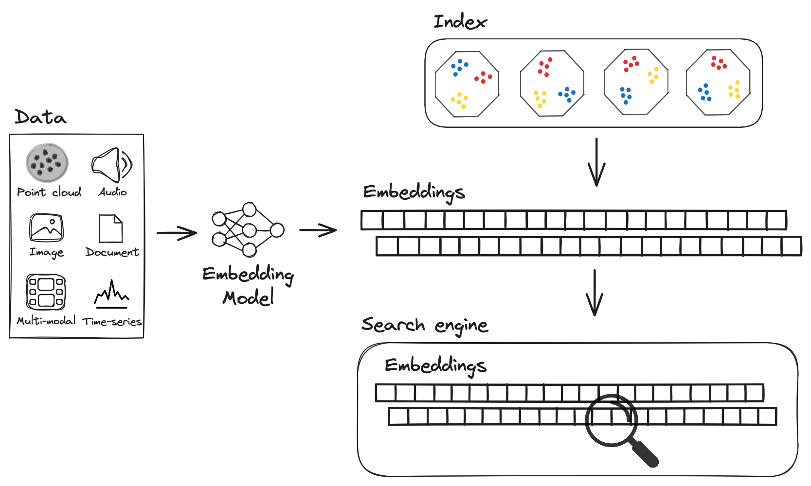
Run a complete example in Python, TypeScript or Rust
Run a complete example in Python, TypeScript or Rust
These examples create a three-row table and find the two closest matches to a
query vector. They use hand-written vectors, so you can try the query without
an embedding model. The temporary table is removed when the program finishes.The first result is the puppy record, whose vector exactly matches the query.
The dog record is next.
- Python: Install with
pip install lancedb, save asvector_search.py, then runpython vector_search.py. - TypeScript: Install with
npm install @lancedb/lancedb, save asvector_search.mts, then runnode vector_search.mtswith Node.js 22.18 or later. - Rust: Download and extract the complete Rust examples, then run
cargo run --locked --bin vector_searchfrom the extracted directory.
_distance is smaller for closer matches. This example
uses an exhaustive scan; the indexing section explains how to search larger tables.Supported distance metrics
A distance metric determines how LanceDB compares vectors. Choose the metric recommended by your embedding model. Use the same metric when building an index and querying it. LanceDB supportsl2, cosine, dot and hamming. An unindexed search uses
l2 by default; Hamming distance is for binary vectors. The table below shows
the value returned in the _distance column. Smaller values rank first.
For indexed search, supported distance metrics vary by index type:
Configure Distance Metric
Without a vector index, searches usel2 by default. You can specify cosine or
dot instead (hamming is supported for IVF_FLAT indexes only).
When a vector index exists, the search metric must match the metric used to build
the index. If you explicitly request a different metric, LanceDB cannot use that
index and falls back to an exhaustive (brute-force) search. On LanceDB Cloud (legacy hosted service), the
brute-force KNN safety limit can reject that search on a large table instead of
executing it. LanceDB Enterprise doesn’t have the limit.
If you omit the search metric, current SDKs use the index metric when an index is
available. Some older SDK versions sent l2 when the metric was omitted; with a
non-l2 index, explicitly set the matching metric or upgrade the SDK.
.limit(...) on vector searches you run in applications. You can page through results with .offset(...) and include LanceDB’s internal row id with .with_row_id() / .withRowId() when an operation requires internal row IDs. Use your own ID column for application identifiers.
Selecting the vector column
If your table has exactly one vector column, you can omit the column name and LanceDB will pick it for you. This works for both top-level columns (such asvector) and vector fields nested inside a struct (such as image.embedding).
When LanceDB can’t infer a single column, it raises a ValueError (Python) or rejects the query (Node/Rust). Two cases trigger this:
- No vector column: the schema has no
fixed_size_listorlistof floats. - Multiple candidates: more than one column matches the query’s dimension. The error lists every candidate path so you can pick one explicitly.
[A-Za-z0-9_] in backticks (for example, `image-meta`.`embedding.v1`).
image.embedding and text.embedding), LanceDB still picks the one whose dimension matches your query vector. If two candidates have the same dimension, you must pass the column name explicitly.
Search with a vector index
An approximate nearest-neighbor (ANN) index narrows the set of vectors examined for a query. It can reduce query latency, but may miss neighbors that an exhaustive search would find. Compare recall and latency on queries that represent your application before choosing an index and its search settings.Exact vs Approximate Distances
When doing vector search, the meaning of “distance” depends on whether you are using an index and whetherrefine_factor is specified as part of your query.
nprobes controls how many partitions are searched to find candidates, approx_mode controls the query-time speed/recall trade-off for RQ-quantized and filtered HNSW indexes, and refine_factor controls how many candidates are rescored on full vectors for better distance fidelity and reranking quality.
The table below summarizes the behavior of _distance in search results based on your query configuration:
Tuning approx_mode
Python 0.41.0 and TypeScript 0.41.0 do not expose this setting. The Python
example baseline is 0.42.0b8; TypeScript exposes
approxMode starting with
0.42.0-beta.1. Rust 0.41.0 already exposes approx_mode. See the
client versions.approx_mode when you want to adjust the speed/recall trade-off for approximate vector search at query time. It applies to RQ-quantized indexes, such as IVF_RQ, and to filtered searches on HNSW indexes. Other index types, and queries that bypass the index, ignore it.
The supported values are:
approx_mode defaults to normal and can change per query without rebuilding the index. The Python and Rust APIs call it approx_mode, and the TypeScript API calls it approxMode. On HNSW, fast enables ACORN traversal only when a filter leaves a non-trivial subset of rows; unfiltered or all-row searches use the regular traversal, and very selective filters may use an exact scan instead. If you also set refine_factor, LanceDB first uses approx_mode while finding candidates, then reranks the selected candidates on full vectors.
Tuning nprobes
For IVF vector indices, start with Auto by leaving the probe settings unset.
LanceDB chooses how many partitions to search to balance recall and latency. It
can search further if a filter leaves too few results, within any limits you set.
The examples below assume table has an IVF index and query_vector uses the
same embedding model and dimension as its vectors.
Python
Adjust speed and recall
Usesearch_effort to tune how much work a search does. It accepts values from
0 to 1; 0.5 uses Auto. Increase it to search more partitions when recall is
too low, or decrease it when you can trade some recall for lower latency.
search_effort(0.95) does not mean 95% recall.
SDK builds using Lance 15.0.0-beta.11 or later provide these calibrated tiers:
The probe budget adapts to the distance metric and requested
k, so you can
keep the same effort when changing the result count. The lower tiers were
calibrated for l2, cosine and dot through k=100000. This is the tested
range, not a limit on k; Hamming and larger requests remain uncalibrated.
These are average routing objectives, not guarantees for each query or final
Recall@k. Quantization, filtering and explicit probe bounds can lower final
recall. Remote queries require a server with the corresponding Lance version;
upgrading only the client does not change server-side routing.
Python
search_effort(1) searches all partitions
and can be expensive. In TypeScript, the method is named searchEffort.
Set probe limits
Use explicit probe counts when you have measured a suitable range for your workload:
Counts apply per index segment, not to the entire query. With many segments,
more probes can mean substantially more data reads and cache-fill writes. A
probe cap is not a limit on total latency or I/O.
Use positive counts and keep the minimum no larger than the maximum. Leave the
maximum unset to allow further searching as needed. If filtered queries return
too few results, raise or remove that cap; see the
bounded-search example.
Python
search_effort overrides nprobes. Explicit min/max bounds still apply;
setting them equal fixes the count.
Check result quality
Auto was tuned toward roughly 95% average recall in benchmark tests. That is a starting point, not a guarantee for your data or every query. Returningk results also does not mean they are the true nearest k neighbors.
Measure recall on representative
queries against an exact search with the same metric and filter. Test the settings
you intend to use: an Auto search capped at 50 probes can search fewer partitions
than fixed nprobes(50), so the two can have different recall.
If more probes stop improving quality, try increasing refine_factor or using
a higher-precision index. More probes do not remove quantization error, and
refinement can only rerank the candidates the search finds.
The Python examples use APIs available in LanceDB 0.41.0. Remote queries need
server support too. Older clients may send fixed probe settings by default;
upgrading the server alone does not switch those requests to Auto.Auto’s calibration covers
l2, cosine and dot searches up to k=100000.
For Hamming or larger requests, measure quality and latency on your workload
before relying on the defaults.Vector Search with Prefiltering
This is the default vector search setting. You can use prefiltering to boost query performance by reducing the search space before vector calculations begin. The system first applies your filter criteria to the dataset, then conducts vector search operations only on the remaining relevant subset.select() to choose the returned
columns and limit() to set the maximum number of results.
Vector Search with Postfiltering
Postfiltering selects vector-search candidates before applying the metadata predicate. It can return fewer matches than requested, even when other rows in the table satisfy the predicate. Use prefiltering when you want the nearest records within the matching subset.Post-filtering in LanceDB applies
the filter condition after obtaining the nearest neighbors based on vector similarity.
Multivector Search
Use multivector search when your documents contain multiple embeddings and you need sophisticated matching between query and document vector pairs. The late interaction approach finds the most relevant combinations across all available embeddings and provides nuanced similarity scoring.np.random.random(size=(2, 256)) creates a 2×256 array with two random query vectors, .limit(5) returns the top 5 best document-query combinations, and .to_pandas() provides results in a DataFrame format.
For the supported metric, how scoring works and a complete example, see the
multivector search walkthrough.
Advanced Search Scenarios
Search With Distance Range
Usedistance_range search when you need vectors within particular similarity bounds rather than just the closest neighbors. The system filters results to only include vectors that fall within your specified distance thresholds from the query.
distance_range() method filters results by similarity thresholds - the first example finds vectors with distance between 0.1 and 0.5, the second finds vectors closer than 0.5, and the third finds vectors farther than 0.1.
Each approach returns Arrow tables with vectors that fall within your specified distance thresholds.
Search With Binary Vectors
Use binary vector search for scenarios involving binary embeddings, such as those produced by hashing algorithms. The system stores these efficiently as packed uint8 arrays and uses Hamming distance calculations to determine vector similarity.np.random.randint(0, 2, size=256) creates binary vectors, np.packbits() compresses them to bytes, and .distance_type("hamming") specifies hamming distance for similarity calculation.
The search produces an Arrow table with binary vectors ranked by how many bits differ from the query.
Scaling Vector Search
Query multiple vectors in a batch
Batch search accepts multiple query vectors in one request. Thequery_index
column identifies which query produced each result. Measure throughput and
latency with your workload when choosing a batch size.
query_index to
associate each row with the corresponding input vector.
Include or skip unindexed rows
To optimize for speed over completeness, enable thefast_search flag in your query to skip searching unindexed data.
By default, search includes both indexed vectors and unindexed rows visible to
the query. LanceDB scans the unindexed rows directly. fast_search skips that
scan, which can reduce query time but omit recent records.
Expected performance at scale
Enterprise At 1 billion rows, LanceDB Enterprise reaches p50 28 ms and p99 58 ms on fully cached data with no custom tuning — a representative floor to plan around, not a ceiling. Measured with 1,536-dimensional embeddings, an IVF-RQ index,nprobe=8, k=100, on the best-performing configuration
tested at that scale. The exact numbers depend on your deployment’s shape
(cluster size, storage class, dataset); for higher performance, talk to
the sales team.
Search without a vector index
Search With No Index
The simplest way to perform vector search is to perform a brute force search, without an index, where the distance between the query vector and all the vectors in the database are computed, with the top-k closest vectors returned. This is equivalent to a k-nearest neighbours (kNN) search in vector space. Choose brute force search when you need guaranteed 100% recall, typically with smaller datasets where query speed isn’t the primary concern. The system scans every vector in the table and calculates precise distances to find the exact nearest neighbors.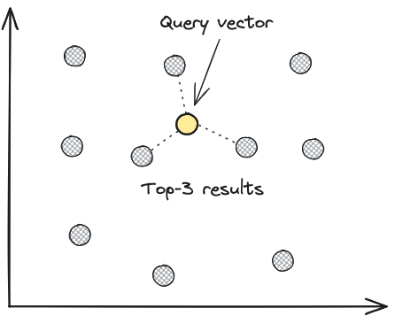
Bypass the Vector Index
Usebypass_vector_index to get exact, ground-truth results by performing exhaustive searches across all vectors. Instead of relying on approximate methods, the system directly compares your query against every vector in the table, ensuring 100% recall at the cost of increased query time.
.bypass_vector_index() method forces LanceDB to perform an exhaustive search through all vectors instead of using the approximate nearest neighbor index, ensuring exact results but at the cost of slower performance.
The query returns the nearest five rows within its filters and distance bounds.
Use an exhaustive scan as a baseline when measuring ANN recall.
This approach is particularly useful when:
- Evaluating ANN index quality
- Calculating recall metrics to tune index parameters
- Ensuring exact results for critical applications
Multivector search walkthrough
LanceDB’s multivector support enables you to store and search multiple vector embeddings for a single item. This capability is particularly valuable when working with late-interaction models like ColBERT and ColPaLi, which generate multiple embeddings per document. In this tutorial, you’ll create a table with multiple vector embeddings per document and learn how to perform multivector search. For more end-to-end examples, see the VectorDB recipes repository.Multivector Support
Each item in your dataset can have a column containing multiple vectors, which LanceDB can efficiently index and search. When performing a search, you can query with either a single vector embedding or multiple vector embeddings. Each query vector must match the inner vector dimension in the multivector column. This applies to both single-vector queries and multi-vector query matrices.Computing Similarity
MaxSim (Maximum Similarity) is a key concept in late-interaction models that:- Computes the maximum similarity between each query embedding and all document embeddings
- Sums these maximum similarities to get the final relevance score
- Effectively captures fine-grained semantic matches between query and document tokens
Using Multivector Search
1. Setup
Connect to a local LanceDB database and import the required libraries.To run this walkthrough on LanceDB Enterprise, connect with
lancedb.connect(uri="db://your-database", api_key="your-api-key", region="your-region")
instead. The remaining steps are the same.2. Define Schema
Define a schema that specifies a multivector field. A multivector field is a nested list structure in which each document contains multiple vectors. In this case, we’ll create a schema with:- An ID field as an integer (int64)
- A vector field that is a list of lists of float32 values
- The outer list represents multiple vectors per document
- Each inner list is a 256-dimensional vector
- Using float32 for memory efficiency while maintaining precision
3. Generate Multivectors
Generate sample data where each document contains multiple vector embeddings, which can represent different aspects or views of the same document. In this example, we create 1024 documents where each document has 2 random vectors of dimension 256, simulating a real-world scenario where you might have multiple embeddings per item.4. Create a Table
Create a table with the defined schema and sample data, which will store multiple vectors per document for similarity search.5. Build an Index
Only cosine similarity is supported for multivector search operations. For faster search, build the standardIVF_PQ index over your vectors:
Indexing matters more for multivector tables than for single-vector ones.A brute-force scan over a multivector column has to compare every query vector to every document vector in every row, so the cost grows with both the row count and the number of vectors per row.
In LanceDB Embedded, the query will just run, so a large unindexed multivector table can stall a process for a long time before returning results.On LanceDB Cloud, the brute-force KNN safety check applies a stricter row threshold to multivector columns; roughly 10× lower than for single-vector columns. So an unindexed multivector table can be rejected with a “vector search would use brute-force KNN” error well before a comparable single-vector table would. LanceDB Enterprise doesn’t have the limit. Build the index before you start hitting it from production traffic, even if the dataset is small enough that you’d skip indexing for a single-vector workload.